Ridge and Valley Surfaces from Volume Data

A C implementation of the grid-based algorithm for ridge and valley surface extraction that has been presented in [STS10] is available in the open source library Teem. This tutorial explains how to use it. Parts of the tutorial are based on example data and code provided by Gordon Kindlmann.

If you are new to Teem, you may find the quick introduction helpful. In particular, it explains how to build a recent developer version from the SVN, needed to use all functions in my code examples. I am using OpenGL to render the extracted surfaces, but this will not be covered here. Instead, please refer to the “red book” [Shr09] to learn about OpenGL. If you should encounter any problems with the code or this tutorial, please contact Teem’s mailing list.

Preparing Your Data

Teem has its own file format, NRRD (Nearly Raw Raster Data). If you look at the NRRD specification, it is straightforward to turn many other raster-based file formats into NRRD by writing a short ASCII header file for them. In this tutorial, we will use the synthetic test dataset mobius-noisy.nrrd that is available for download here. It is due to Gordon Kindlmann and can be re-created on the command line:

teem/src/nrrd/test/genvol -s 40 40 40 \
  | unu crop -min 4 0 12 -max M-4 M M-12 \
  | unu 2op nrand - 0.85 \
  | unu 2op + - 3 \
  | unu resample -s x1 x1 x1 -k cubic:1,1,0 \
  | unu 2op / - 83 -o mobius-noisy.nrrd

Memory Management

This tutorial tries to promote error checking and memory management; for the latter, we will use a cleanup mechanism in Teem that is called “mop”:

#include <teem/air.h>
airArray *mop = airMopNew();

The mop can be given pointers to memory that you would like to free at the end of your code. Before exiting because of an error, you would simply call

airMopError(mop);

to release the allocated memory. If things went smoothly, but you still want to free the memory, you call

airMopOkay(mop);

Extracting The Surface

The surface extraction code is in the Teem module seek:

#include <teem/seek.h>

Extraction requires three steps: Loading the data, defining the interpolation, and setting the parameters of the extraction algorithm itself. Loading the data works like this:

const char *filename = "mobius-noisy.nrrd";
Nrrd *nin = nrrdNew();
if (nrrdLoad(nin, filename, NULL)) {
  char *err;
  airMopAdd(mop, err = biffGetDone(NRRD), airFree, airMopAlways);
  fprintf(stderr, "ERROR: Could not open input file \"%s\"\n"
          "Reason: %s\n", filename, err);
  airMopError(mop); return 1;
}
airMopAdd(mop, nin, (airMopper)nrrdNuke, airMopAlways);

Gage is used to make convolution-based measurements in your input. We will tell it to use a second-order continuous cubic B-spline as the interpolation kernel and to measure all quantities needed for crease extraction, including Hessian eigenvectors and -values:

gageContext *gctx = gageContextNew();
airMopAdd(mop, gctx, (airMopper)gageContextNix, airMopAlways);
double kparm[3]={1, 1.0, 0.0}; /* parameters of the cubic kernel */
gagePerVolume *pvl;
if (!(pvl = gagePerVolumeNew(gctx, nin, gageKindScl))
    || gagePerVolumeAttach(gctx, pvl)
    || gageKernelSet(gctx, gageKernel00, nrrdKernelBCCubic, kparm)
    || gageKernelSet(gctx, gageKernel11, nrrdKernelBCCubicD, kparm)
    || gageKernelSet(gctx, gageKernel22, nrrdKernelBCCubicDD, kparm)
    || gageQueryItemOn(gctx, pvl, gageSclNormal)
    || gageQueryItemOn(gctx, pvl, gageSclHessEval)
    || gageQueryItemOn(gctx, pvl, gageSclHessEvec)
    || gageQueryItemOn(gctx, pvl, gageSclHessEval2) /* ridge strength */
    || gageUpdate(gctx)) {
  char *err;
  airMopAdd(mop, err = biffGetDone(GAGE), airFree, airMopAlways);
  fprintf(stderr, "ERROR while setting up Gage:\n%s\n", err);
  airMopError(mop); return 1;
}

Now, we can set up the extraction itself:

double strength=150;
seekContext *sctx = seekContextNew();
airMopAdd(mop, sctx, (airMopper)seekContextNix, airMopAlways);
int E=0;
if (!E) E |= seekDataSet(sctx, NULL, gctx, 0);
if (!E) E |= seekItemGradientSet(sctx, gageSclGradVec);
if (!E) E |= seekItemEigensystemSet(sctx, gageSclHessEval, gageSclHessEvec);
if (!E) E |= seekItemHessSet(sctx, gageSclHessian);
if (!E) E |= seekItemNormalSet(sctx, gageSclNormal);
if (!E) E |= seekStrengthUseSet(sctx, AIR_TRUE);
if (!E) E |= seekStrengthSet(sctx, -1, strength);
if (!E) E |= seekItemStrengthSet(sctx, gageSclHessEval2);
if (!E) E |= seekNormalsFindSet(sctx, AIR_TRUE);
if (!E) E |= seekTypeSet(sctx, seekTypeRidgeSurfaceT);

The strength parameter filters out unimportant creases and needs to be adjusted for the individual dataset; in our example, strength=150 works pretty well. The mathematical definition of a crease surface corresponds to strength=0, but in practice, such a low value will lead to a hopeless amount of clutter (try it, if you want). We are now ready to trigger surface extraction:

limnPolyData *pld = limnPolyDataNew();
if (!E) E |= seekUpdate(sctx);
if (!E) E |= seekExtract(sctx, pld);
if (E) {
  char *err;
  airMopAdd(mop, err = biffGetDone(SEEK), airFree, airMopAlways);
  fprintf(stderr, "ERROR during surface extraction:\n%s\n", err);
  airMopError(mop); return 1;
}

Finally, pld contains everything you need in order to render the surface as triangle soup: Vertex positions in xyzw, normals in norm, an index array in indx. Obviously, the surface is non-orientable, so you have to discard the sign of the normals for shading (in OpenGL, I’m doing this with a trivial vertex shader; see [RLC09] for more information on the OpenGL shading language). The result should look like this:

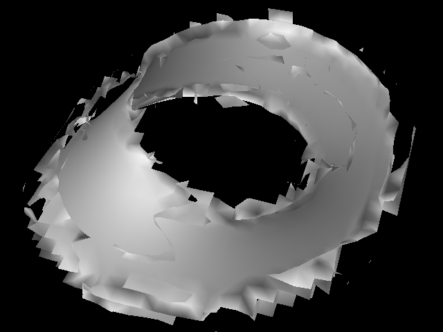
This ridge extraction result is still preliminary.

See those ugly zigzag edges and artifacts? They indicate that extraction is not yet complete, so be sure to follow the next Section of this page, on post-filtering!

Additional hints:

• The above code extracts intensity ridges from a scalar field. If you need valleys, replace seekTypeRidgeSurfaceT with seekTypeValleySurfaceT; gageSclHessEval2 with gageSclHessEval0 in the definition of strength; and -1 with 1 in seekStrengthSet. The value of strength itself is always positive, no matter if you are extracting ridges or valleys.
• If you have vector- or tensor-valued input (e.g., if you try to compute FA ridges in a second-order tensor field [KTW07]), you need to replace gageKindScl with the appropriate gageKind (e.g., tenGageKind) and choose suitable gageItems (e.g., tenGageFANormal etc.).
• Calling airMopOkay after the above code will not free the result in pld. I’m assuming that you want to keep it.

Post-Filtering

Post-filtering is strictly required to trim the mesh boundaries and to clean up some spurious triangles. For this cleanup, do:

Nrrd *nval = nrrdNew();
airMopAdd(mop, nval, (airMopper) nrrdNuke, airMopAlways);
if (1==seekVertexStrength(nval, sctx, pld)) {
  char *err;
  airMopAdd(mop, err = biffGetDone(SEEK), airFree, airMopAlways);
  fprintf(stderr, "ERROR during surface probing:\n%s\n", err);
  airMopError(mop); return 1;
}
limnPolyDataClip(pld, nval, sctx->strength);

After this step, the result should look like this:

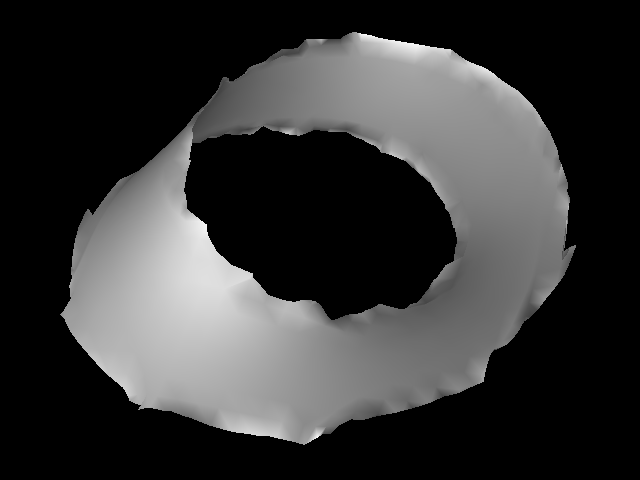
The cleanup has removed spurious surface patches and trimmed boundaries.

One reason for doing this in a separate step, rather than integrating it into the main extraction routine, is that it allowed me to keep the code simpler. Another benefit is that this cleanup is easily and efficiently combined with any application-specific post-filtering that you might want to apply. Telling from my own experience and from what I understand from the literature, such additional filtering is required in most real-world applications of crease surfaces. Filtering the mesh by multiple criteria simultaneously (strength should always be one of them) is implemented in limnPolyDataClipMulti.

Scale and Pre-Filtering

The ridge in our example dataset exists at a small scale. This means that it is narrow with respect to the sampling rate. If you look at a cross-sectional slice through the dataset, you’ll notice that the ridge is few voxels wide, and that its intensity drops off rapidly away from the center:

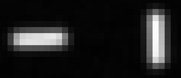
Looking at the example data shows that the ridge is few voxels wide.

My algorithm looks for creases at a fixed and fine scale. If you are looking for larger-scale (wider) ridges or valleys, you might find that they are not reconstructed correctly. In this case, it will help to pre-filter (i.e., blur) your data before extracting creases. This will get rid of small-scale (and potentially noise-related) creases and help to more reliably find the larger-scale ones. Gaussian convolution is widely used for pre-filtering creases.

If you are looking for creases at different scales, in the same dataset, you will have to apply non-uniform pre-smoothing (i.e., blur more in regions of large-scale features, less where detail is to be preserved). More sophisticated methods for multiscale crease extraction will try to determine and apply the required amount of local smoothing automatically, or can even find spatially intersecting creases at different scales. However, this comes at a considerable computational expense. Teem features a method for scale-aware crease extraction that is based on particle systems [KSJ09]; Gordon offers a tutorial for this.

Using a Virtual Grid

A widely used trick to get a more accurate result is to extract the surface on a refined grid. In most cases (such as the one above), this should no longer be needed with my algorithm. However, if you are interested in fine-scale surface features or if you should encounter show-stopping artifacts, you can specify a virtual grid resolution via:

size_t samples[3];
ELL_3V_SET(samples,
           2*nin->axis[0].size, 2*nin->axis[1].size, 2*nin->axis[2].size);
if (!E) E |= seekSamplesSet(sctx, samples);

This code doubles the resolution in each dimension, so computation takes approximately eight times as long, and almost four times as many triangles are used. Often, more subtle refinements (such as factor sqrt(2), which roughly doubles the triangle count) already lead to much improved results, at a more moderate cost.

Just in case you should want to compare my method to the previous state of the art, you are welcome to replace seekTypeRidgeSurfaceT with seekTypeRidgeSurface or seekTypeRidgeSurfaceOP. This activates two algorithms that were widely used before [STS10]. You will find that you need to combine them with a much finer virtual grid to obtain comparable quality.

When using crease surfaces in applications, it is important to remember that no existing algorithms for their extraction make any guarantees on the correctness of their results. Crease surface extraction is a much harder problem than isosurface extraction, and still not fully solved!

Caveat on Non-Generic Data

Since our paper is concerned with generic properties of crease surfaces (cf. Section 3 in [STS10]), my implementation assumes generic input data. This means that it does not support branchings or crease surfaces that exactly intersect a voxel corner.

It is very unlikely that this will be a source of problems if you run the algorithm on real data, since most real-world data is generic. In fact, in unconstrained scalar fields, branchings or exact intersections of voxel corners occur with probability zero and even if you deliberately construct an example with these properties, they can be removed by an arbitrarily small perturbation.

However, even seemingly simple synthetic examples might result in non-generic input. If the algorithm seems to behave strangely on a synthetic example, try if adding a small amount of random noise removes the problem. By the way, a very similar problem exists with standard isosurfacing algorithms: They are typically not able to extract self-intersecting isosurfaces. Again, self-intersecting level sets are non-generic, but can easily be constructed in synthetic data.

Surface Normals

The surface normals in the example above are computed analytically, from the values in the given scalar field. This is described in Section 4.4 of [STS10]. It usually works pretty well, but can lead to less-than-ideal results at surface boundaries. If you should prefer to approximate normals from the mesh, an algorithm for that, suitable for non-orientable surfaces, is available in limnPolyDataVertexNormalsNO().

References

[KSJ09]

Gordon Kindlmann, Raul San Jose Estepar, Stephen M. Smith, and Carl-Fredrik Westin. Sampling and Visualizing Creases with Scale-Space Particles. IEEE Transactions on Visualization and Computer Graphics 15(6):1415-1424, 2009

[KTW07]

Gordon Kindlmann, Xavier Tricoche, and Carl-Fredrik Westin. Delineating White Matter Structure in Diffusion Tensor MRI with Anisotropy Creases. Medical Image Analysis 11(5):492-502, 2007

[RLC09]

Randi J. Rost and Bill Licea-Kane. OpenGL Shading Language (3rd edition). Addison-Wesley, 2009

[Shr09]

Dave Shreiner. OpenGL Programming Guide: The Official Guide to Learning OpenGL, Versions 3.0 and 3.1 (7th edition). Addison-Wesley, 2009.

[STS10]

(1, 2, 3, 4) Thomas Schultz, Holger Theisel, and Hans-Peter Seidel. Crease Surfaces: From Theory to Extraction and Application to Diffusion Tensor MRI. IEEE Transactions on Visualization and Computer Graphics 16(1):109-119, 2010